Basic Concepts

Quantum Circuits

In quantum computing, a quantum circuit represents a sequence of operations that are intended to be applied to qubits.

Let's start with an example. We are going to start by importing Snowflurry.

using Snowflurry

We can then create an empty QuantumCircuit by specifying the number of qubits (qubit_count) and classical bits (bit_count) the circuit will involve. The classical bits (or result bits) are ordinary memory registries that each store the output of a Readout operation on a particular qubit.

c = QuantumCircuit(qubit_count = 2, bit_count = 2)
# output
Quantum Circuit Object:
   qubit_count: 2 
   bit_count: 2
q[1]:
     
q[2]:

Optionally, if bit_count is not specified it will assume the same value as qubit_count.

c = QuantumCircuit(qubit_count = 2)
# output
Quantum Circuit Object:
   qubit_count: 2 
   bit_count: 2
q[1]:
     
q[2]:

You can visualize a QuantumCircuit object at any point by simply printing it:

print(c)
# output
Quantum Circuit Object:
   qubit_count: 2 
   bit_count: 2
q[1]:
     
q[2]:

We have not yet added any quantum operation to our circuit and it looks empty! So, let's add some quantum operations!

Quantum Gates

Basic logical operations on qubits are commonly called quantum logic gates or simply gates. We will quite often talk about single-qubit gates, two-qubit gates or multiple-qubit gates in quantum information theory.

Let's start by adding a single-qubit gate called the Hadamard gate to our circuit, c, and specify that it will only operate on qubit '1'. The Hadamard gate is one of the most frequently used gates in quantum computing as it puts its target qubit into a perfect superposition of state $\left|0\right\rangle$ and $\left|1\right\rangle$.

We build this gate by calling hadamard() function with the target qubit = 1, and we add it to our circuit c by calling the push! function:

push!(c, hadamard(1))
# output
Quantum Circuit Object:
   qubit_count: 2 
   bit_count: 2
q[1]:──H──
          
q[2]:─────

Note the exclamation mark at the end of push! which emphasizes the fact that we have called a mutating function that will change the argument c (our quantum circuit).

If we now print circuit c, we will see the following output

print(c)
# output
Quantum Circuit Object:
   qubit_count: 2 
   bit_count: 2
q[1]:──H──
          
q[2]:─────

Now let's add a famous two-qubit gate, control_x, also known as the CNOT gate in the quantum information community. Here the first argument is the control_qubit = 1, and the second is the target_qubit = 2.

push!(c, control_x(1, 2))
# output
Quantum Circuit Object:
   qubit_count: 2 
   bit_count: 2 
q[1]:──H────*──
            |  
q[2]:───────X──

Voilà! You just made your first quantum circuit with Snowflurry that does something interesting.

It puts a two-qubit register in a maximally-entangled quantum state ($\frac{\left|00\right\rangle+\left|11\right\rangle}{\sqrt{2}}$). (The qubit ordering convention used is qubit number 1 on the left, with each following qubit to the right of it.) This state is one of the four celebrated Bell States or the EPR states. These states do not have classical counterparts and are among the building blocks of many interesting ideas in quantum computing and quantum communication.

Circuit Simulation

You can verify what your circuit will ideally do on a real computer by simulating the circuit on your own local machine:

simulate(c)
# output
4-element Ket{ComplexF64}:
0.7071067811865475 + 0.0im
0.0 + 0.0im
0.0 + 0.0im
0.7071067811865475 + 0.0im

The output of the simulate() function is a Ket object. A Ket is a complex vector that represents the wavefunction of a quantum object such as our two-qubit system.

Histogram

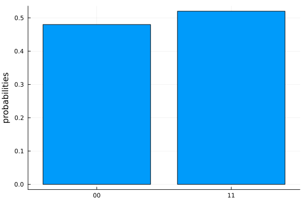
In the previous section, we used the simulate function to calculate the wavefunction of a two-qubit quantum register, after the circuit, c, is applied to it. However, in the real world, we do not have direct access to the wavefunction of a quantum register. Rather, we need to run the quantum circuit several times over (several shots) on the quantum processor and measure the qubits states at the end of each shot. The result of each shot is a bitstring that tells us which qubits were measured to be in state $\left|0\right\rangle$ and which qubits were measured to be in state $\left|1\right\rangle$. The probability of getting a bitstring then depends on the wavefunction.

We can indeed mimick this behaviour in our simulations as well. This can be achieved by using the plot_histogram function from the SnowflurryPlots library. For example, we can generate a histogram which shows the measurement output distribution after taking running the circuit c for a given number of shots, let's say 100 times, on a quantum computer simulator:

using SnowflurryPlots
push!(c, readout(1, 1), readout(2, 2))
plot_histogram(c, 100)

In the next tutorial, we will discuss how to run the above circuit on a virtual quantum processor.